If you’re spending way too long on repetitive data tasks in Google Sheets, you’re not alone. I used to lose hours every week to the same old steps—until I stumbled on a single function that did the heavy lifting for me. Let me introduce you to the QUERY function.

5

Automated Sorting That Updates Itself in Real-Time

The most immediate way the QUERY function improved my spreadsheets is by eliminating my constant re-sorting headaches. You know that frustrating cycle where you sort your data, then an hour later, new information comes in, and suddenly your sorted list is completely out of order again. That’s the one.

Say you want to track your company’s inventory by price. Instead of re-sorting endlessly, you can use a QUERY like this:

=QUERY(A:G, "SELECT * ORDER BY E desc")

In this example, you’re telling Google Sheets to pull everything from columns A through G and sort it by column E (which holds prices, in this case) in descending order.

Immediately, your most expensive cars float straight to the top.

What makes this a game-changer is that it doesn’t stop working. When a new $250,000 car gets added to your spreadsheet, it instantly appears at the top of your QUERY results. No need to sort again.

What used to take me several minutes of clicking and dragging throughout the day now happens automatically. More importantly, I never miss high-priority items anymore because they’re always right where they should be.

4

Combining Multiple Steps Into One Formula

I can’t tell you how many times I used to find myself doing this dance: filtering the data, sorting it, hiding certain columns, and maybe grouping things together. Now, thanks to QUERY, I can do all of that in one shot.

Let’s say I want to prepare a sales review, and I need to do the following:

• Filter out only the sold cars
• Remove any cars under $30,000
• Exclude the Teslas
• Sort by price to see the biggest sales first

That’s four separate steps. If I had to do this manually and make a mistake anywhere, I’d have to start afresh. Instead, I type:

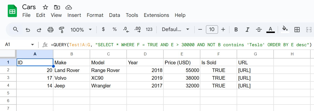
=QUERY(Test!A:G, "SELECT * WHERE F = TRUE AND E > 30000 AND NOT B contains 'Tesla' ORDER BY E desc")

One formula replaces four steps. Because I inserted the QUERY function on a blank sheet, I added the sheet’s name with an exclamation mark (Test!) before specifying the columns with my data.

The best part is that I can get even fancier with clauses like PIVOT, LABEL, etc. For instance, when I need to see how each year’s offerings are selling, I add GROUP BY:

=QUERY(Test!A:G, "SELECT D, SUM(E) WHERE F = TRUE GROUP BY D ORDER BY SUM(E) desc")

This shows me the revenue so far from each year’s releases, automatically sorted from highest to lowest.

The time savings add up fast. What used to take me 10–15 minutes of clicking, filtering, and organizing now takes 30 seconds to type a formula. And unlike my old multistep process, I never accidentally skip a step or mess up the order.

Related

These 8 Google Sheets Formulas Simplify My Budgeting Spreadsheet

Why crunch numbers manually when Google Sheets can do the heavy lifting?

3

Handling Massive Datasets Without Any Lag

Picture this: You’re trying to find your most recent 100 customers from a database of over 50,000 rows to send a targeted email campaign. That’s simple enough, right?

Wrong. Every time you attempt sorting, filtering, or maneuvering that kind of massive dataset, Google Sheets will likely freeze. I dealt with this until I discovered QUERY could handle bulky datasets.

Here’s an example:

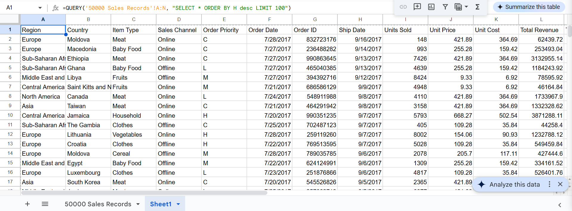
=QUERY('50000 Sales Records'!A:N, "SELECT * ORDER BY H desc LIMIT 100")

The first formula will grab the top 100 most recent shipments, as column H includes shipment dates. Meanwhile, the second one will grab orders 61 through 160.

Instead of making your computer process and display all 50,000+ rows, while taking its sweet time, just so you can look at the top 100, QUERY (with the LIMIT and OFFSET clause) is smart enough to grab exactly what you need and leave the rest alone.

You can even use LIMIT and OFFSET with all the other QUERY features—grouping, sorting, filtering—without fighting your browser and wasting time.

Related

My Quest to Find the Perfect Browser on Windows

If only it was simple.

2

Analyzing Data Across Multiple Sheets or Files

Are you still manually copying data between spreadsheets or workbooks just to do one report? You can stop now. QUERY enables you to analyze data across multiple sheets—or even across entirely different files—without ever touching Ctrl+C.

Combine Multiple Tabs in One Go

Say you’ve got quarterly data split across tabs like Sales_Q1 and Sales_Q2, you can merge them into a single dataset using curly brackets. Then, run your analysis just like you would on a single sheet.

=QUERY({Sales_Q1!A:N; Sales_Q2!A:N; Sales_Q3!A:N; Sales_Q4!A:N}, "SELECT Col3, Col1, SUM(Col9) WHERE Col5 = 'C' GROUP BY Col3, Col1")

Let’s say column 3 (Col3) is the Item Type, column 1 the Region, column 9 the Units Sold, and column 5 the Order Priority. Just make sure the structure (columns) of each sheet matches, and you’re good to go.

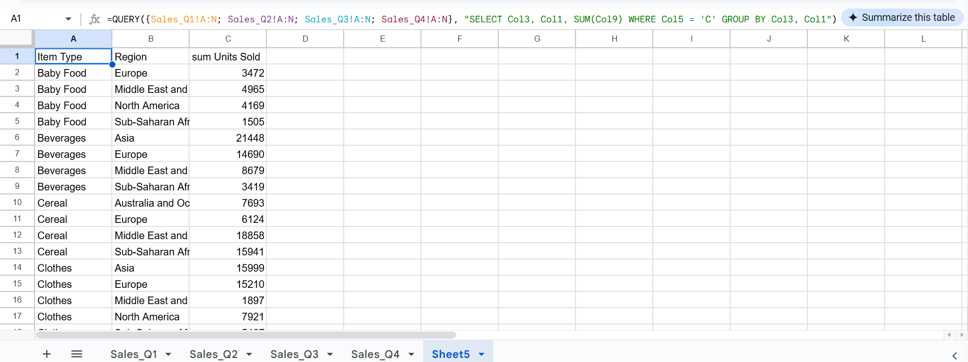
I just combined four sheets with data from different quarters in order to get the total units sold per item and region for C priority orders. Easy peasy!

Pull Data From Another Google Spreadsheet (No Download Required)

If you need data from a completely different file, you can use IMPORTRANGE with Query to bring it in. Say you want to bring in data from our car sales and juxtapose it with the data we’ve gotten from the four sheets, you can use this formula:

=QUERY(IMPORTRANGE(" "Test!A:G"), "SELECT Col4, SUM(Col5) GROUP BY Col4")

You’ll need to grant permission before you can pull data from the external spreadsheet.

Once you grant access, you can grab data from the external spreadsheet in real time, and it’ll update if the source data changes.

QUERY lets you analyze data across tabs and files without having to open a second tab or file.

1

Sorting and Filtering Without Rewriting Formulas

Want to sort or filter your data differently without rewriting your entire QUERY formula every single time? You can, with a simple setup using double quotes and ampersands:

=QUERY({Sales_Q1!A:N; Sales_Q2!A:N; Sales_Q3!A:N; Sales_Q4!A:N}, "SELECT * WHERE Col1 = '"&G21&"'", 1)

When your boss wants to see European data, you just type “Europe” in cell G21.

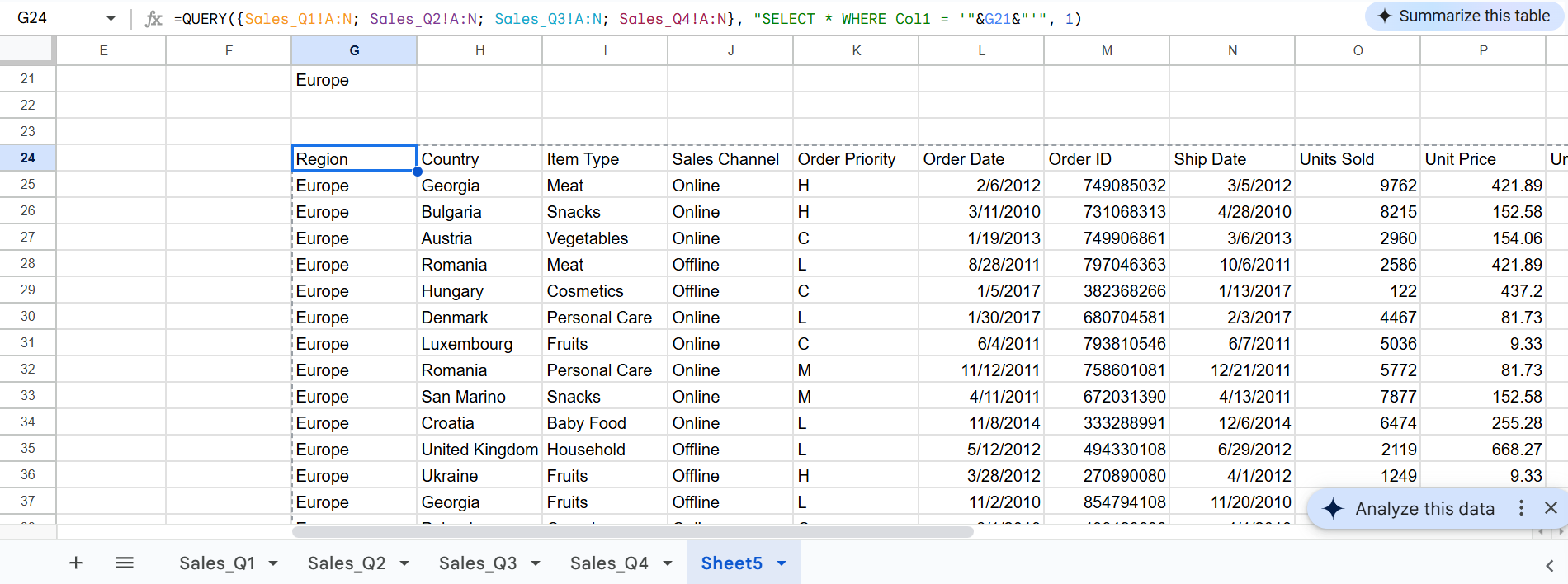
When he wants Sub-Saharan Africa data, you type “Sub-Saharan Africa.” Just ensure it’s a valid entry in column 1. The formula stays the same, but the results update instantly. Once you get the hang of it, it’s incredibly powerful.

The real magic happened when I started using this for date ranges. Dates in QUERY formulas are notoriously picky. They need to be in exactly the right format (YYYY-MM-DD) or everything breaks. But with cell references, you can set up user-friendly date controls:

=QUERY({Sales_Q1!A:N; Sales_Q2!A:N; Sales_Q3!A:N; Sales_Q4!A:N}, "SELECT * WHERE Col6 >= date '"&TEXT(G142, "yyyy-mm-dd")&"' AND Col6

Now, I have Cell G142 for the start date, Cell I142 for the end date, and Column 6 representing the Order Date Column. When someone asks what our sales were from March 15th, 2011, to April 30th, 2015, I just change those two cells instead of wrestling with formula syntax.

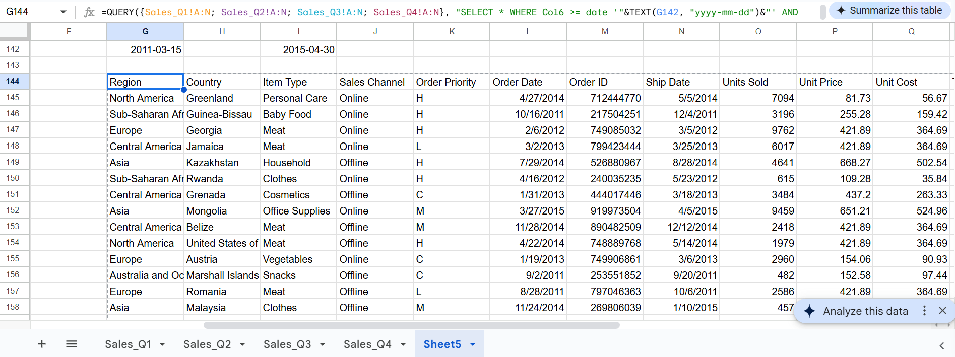
The best part is, I can share these spreadsheets with colleagues who aren’t formula experts. They see clean input cells where they can change the region or adjust date ranges, and they have no idea there’s a complex QUERY running behind the scenes.

Related

The Top 6 Excel Formulas Every Office Worker Should Know

Once you learn these formulas, you’ll wonder how you ever worked without them.

The QUERY function in Google Sheets isn’t just a formula. It’s a full-blown data automation powerhouse. Whether you’re wrangling tens of thousands of rows, copying data between sheets, or just sick of repetitive sorting and filtering, QUERY handles it all with ease (and style).

It’s fast. It’s flexible. And once you start using the QUERY function in Google Sheets, you’ll seriously wonder how you ever managed without it.